set up notebook
In [1]:
#!rm genomes/tb927_6/*
In [2]:
#reload when modified
%load_ext autoreload
%autoreload 2
#activate r magic
%load_ext rpy2.ipython
%matplotlib inline
In [13]:
import os
import pandas as pd
import numpy as np
import matplotlib.pyplot as plt
import seaborn as sns
import utilities as UT
import missingno as msno
import random
import matplotlib.pyplot as plt
import matplotlib.patches as patches
import gc

random.seed(1976)
np.random.seed(1976)
Data Anaylsis
Experiment SetUp
In [14]:
from IPython.display import Image
In [ ]:
In [15]:
#create a dictionary of gene to desc
#from the gff file
def make_desc(_GFF):
    gff =pd.read_csv( _GFF, sep='\t', header=None, comment='#')

    gff = gff[gff.iloc[:,2]=='gene']
    #print( gff[gff[gff.columns[-1]].str.contains('Tb427_020006200')] )
    desc = {}
    for n in gff.iloc[:,-1]:
        n=n.replace('%2C',' ')
        item_list = n.split(';')
        #print (item_list)
        temp_dict = {}
        for m in item_list:
            #print(m)
            temp_dict[m.split('=')[0].strip()]=m.split('=')[1].strip()
        #print(temp_dict['ID'])
        #print(temp_dict['description'])
        desc[temp_dict['ID']]=temp_dict.get('description','none')
    return desc

desc_dict = make_desc('genomes/tb927_3/tb927_3.gff')
desc_dict['Tb10.v4.0073']
Out[15]:
In [16]:
exp = 'P{life_stage}{replica}'
list_df = [exp.format(
    life_stage=life_stage,
    replica=replica)
 for life_stage in ['1','2','3']
 for replica in ['C','T']
            ]
list_df = [n+'/res/'+n+'/counts.txt' for n in list_df]
list_df =[pd.read_csv(n,index_col=[0],comment='#',sep='\t') for n in list_df]
df = list_df[0].copy()
for temp_df in list_df[1:]:
    df = df.join(temp_df.iloc[:,-1])
df.head()
#temp_df = pd.read_csv('BSF/tb927_3_ks_counts_final.txt',index_col=[0],comment='#',sep='\t')
Out[16]:
In [17]:
#df = pd.read_csv('InData/tb927_3_ks_counts_final.txt',index_col=[0],comment='#',sep='\t')
#df.head()
#data_col = df.columns[6:25]
In [18]:
data_col = df.columns[5:]
data_col
Out[18]:
In [19]:
indata = df[data_col]
indata.columns = [n.split('/')[3] for  n in indata.columns]
indata = indata[['P1C','P2C','P3C','P1T','P2T','P3T']]
indata.head()
Out[19]:
In [20]:
print(indata.shape)
indata=indata.dropna()
print(indata.shape)
#indata.loc['KS17gene_1749a']
#indata['desc']=[desc_dict.get(n,'none') for n in indata.index.values]
#indata.to_csv('indata.csv')
#indata.head()
#indata.loc['mainVSG-427-2']
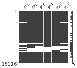
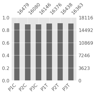
Missing Data Viz
In [ ]:
In [22]:
msno.matrix(indata.replace(0,np.nan).dropna(how='all'),figsize=(4, 4))
Out[22]:
In [23]:
msno.bar(indata.replace(0,np.nan).dropna(how='all'),figsize=(4, 4))
Out[23]:
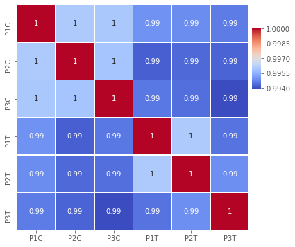
QC - Corr analysis
In [24]:
!mkdir -p Figures
In [27]:
fig,ax=plt.subplots(figsize=(6,6))
cbar_ax = fig.add_axes([.91, .6, .03, .2])
sns.heatmap(np.log2(indata).corr(),
            #vmin=-1,
            cmap='coolwarm',
            annot=True,linewidths=.5,ax=ax, cbar_ax = cbar_ax, cbar=True)
print(ax.get_ylim())
ax.set_ylim(6,0)
plt.savefig('Figures/Figure_2.png')
plt.show()
In [ ]:
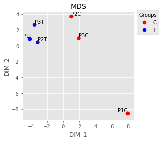
QC - MSD
In [28]:
plt.style.use('ggplot')
palette = ['r']*3+['b']*3
fig,ax = plt.subplots(figsize=(4,4), ncols=1, nrows=1)
UT.make_mds(np.log2(indata),palette,ax,color_dictionary={'r':'C','b':'T',
                                                        })
plt.savefig('Figures/Figure_3.png')
plt.show()
Compute Length and GC content
In [29]:
!mkdir -p InData
In [30]:
!gtf2bed < genomes/tb927_6/tb927_6.gtf > tb927_6.bed
!bedtools nuc -fi genomes/tb927_6/tb927_6.fa -bed tb927_6.bed >InData/GC_content_927.txt
In [31]:
#!bowtie2-build genomes/tb927_5/tb927_5.fa genomes/tb927_5/tb927_5
In [32]:
def get_gene_ids(n):
    res = {}
    temp = n.split(';')
    temp =[n.strip() for n in temp if len(n)>2]
    for f in temp:
        key = f.split(' ')[0]
        value = f.split(' ')[1]
        key=key.replace('\"','').replace('\'','').strip()
        value=value.replace('\"','').replace('\'','').strip()
        res[key]=value
    return res['gene_id']
In [33]:
gc_content = pd.read_csv('InData/GC_content_927.txt',sep='\t')
gc_content = gc_content[gc_content['8_usercol']=='transcript']
gc_content['gene_id'] = [get_gene_ids(n) for n in gc_content['10_usercol']]
gc_content = gc_content.drop_duplicates('gene_id')
gc_content.set_index('gene_id',inplace=True)
gc_content=gc_content[['19_seq_len','12_pct_gc']]
gc_content.columns = ['length', 'gccontent']
gc_content.head()
Out[33]:
In [34]:
indata.head()

#indata.astype(int).to_csv('indata.csv',index=True)
Out[34]:
In [35]:
#metadata=pd.DataFrame()
#metadata['samples']=indata.columns
#metadata['treatment']=['C','C','C','D','D','D','DF','DF','DF','F','F','F']
#metadata['batch']=1
#metadata.reset_index().to_csv('metadata.csv')
In [36]:
print(indata.shape)
indata=indata.join(gc_content,how='inner')
gc_content = gc_content[['length', 'gccontent']]
indata.drop(['length', 'gccontent'],axis=1,inplace=True)
In [ ]:
In [ ]:
In [37]:
#indata.loc['mainVSG-427-2']
edgeR to filter low counts
In [38]:
%%R -i indata
options(warn=-1)
library("limma")
library("edgeR")
head(indata)
In [40]:
%%R
group <- factor(c(
    'C','C','C',
    'T','T','T'
))

y <- DGEList(counts=indata,group=group)
keep <- filterByExpr(y)
y <- y[keep,,keep.lib.sizes=FALSE]
counts = y$counts
genes = row.names(y)
In [41]:
%R -o counts,genes
indata = pd.DataFrame(counts,index=genes,columns=indata.columns)
indata.shape
Out[41]:
In [ ]:
In [42]:
indata=indata.join(gc_content,how='inner')
indata.shape
Out[42]:
GC / length content
In [43]:
gc_content = indata[['length', 'gccontent']]
indata.drop(['length', 'gccontent'],axis=1,inplace=True)
print(indata.shape,gc_content.shape)
indata.head()
Out[43]:
size factors
In [44]:
sizeFactors=indata.sum()
sizeFactors = sizeFactors.values
sizeFactors
Out[44]:
In [45]:
#np.log2(gc_content['length']/1000).plot(kind='hist')
Bias Correction
In [47]:
%%R -i gc_content,indata,sizeFactors
library(cqn)
library(scales)
In [48]:
%%R
stopifnot(all(rownames(indata) == rownames(gc_content)))
cqn.subset <- cqn(indata, lengths = gc_content$length,
                  x = gc_content$gccontent, sizeFactors = sizeFactors,
                  verbose = TRUE)
In [49]:
#%R cqn.subset
Viz Bias
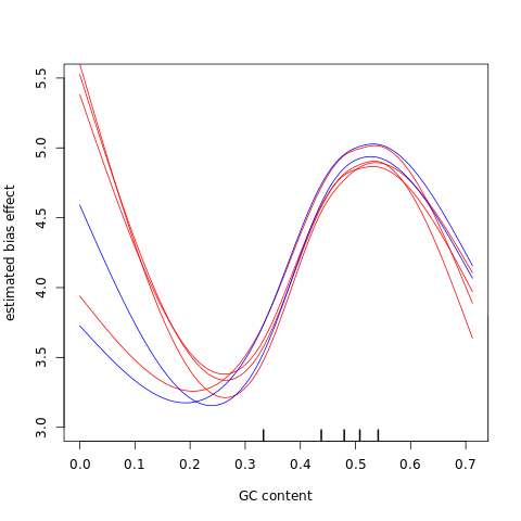
In [50]:
%%R
cqnplot <- function(x, n = 1, col = "grey60", ylab="estimated bias effect",
                    xlab = "", type = "l", lty = 1, ...) {
    if(class(x) != "cqn")
        stop("'x' needs to be of class 'cqn'")
    if(n == 1) {
        func <- x$func1
        grid <- x$grid1
        knots <- x$knots1
    }
    if(n == 2) {
        if(is.null(x$func2))
            stop("argument 'x' does not appear to have two smooth functions (component 'func2' is NULL)")
        func <- x$func2
        grid <- x$grid2
        knots <- x$knots2
    }


    #par(mar=c(5.1, 4.1, 4.1, 8.1), xpd=TRUE)
    matplot(replicate(ncol(func), grid), func, ylab = ylab, xlab = xlab, type = type,
            col = col, lty = lty, ...)

    legend("bottomleft", legend = colnames(x$counts), inset=c(1,0),
           title="Samples", lty = lty, col = col)
    rug(knots, lwd = 2)
    invisible(x)

}


library(repr)
#options(repr.plot.width = 10, repr.plot.height = 0.75)
# Change plot size to 4 x 3
#options(repr.plot.width=4, repr.plot.height=3)


colors <- c(
    'red','red','red','red',
    'blue','blue','blue',
    'green','green','green',
    'yellow','yellow','yellow'
           )
lty =c(1,1,1,
       1,1,1,
      1,1,1,
      1,1,1)

#png("Figures/Figure_12.png")
#par(mfrow=c(1,2))
cqnplot(cqn.subset, col=colors,
        n = 1, xlab = "GC content", lty = lty,
        ylim = c(3, 5.5),

       )
#dev.off()

#ggsave('plot.png', width=8.27, height= 11.69) #A4 size in inches
#dev.off()
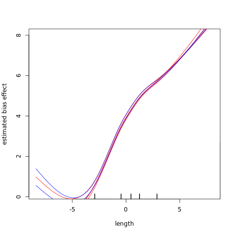
In [51]:
%%R
library(repr)
#options(repr.plot.width = 12, repr.plot.height = 0.75)
# Change plot size to 4 x 3
#options(repr.plot.width=8, repr.plot.height=3)


colors <- c(
    'red','red','red','red',
    'blue','blue','blue',
    'green','green','green',
    'yellow','yellow','yellow'
           )
lty =c(1,1,1,
       1,1,1,
      1,1,1,
      1,1,1)

#par(mfrow=c(1,2))
#png("Figures/Figure_13.png")
cqnplot(cqn.subset, col=colors,
        n = 2, xlab = "length", lty = lty,
        ylim = c(0.2,8),

       )
#dev.off()
Bias Correction
In [52]:
%%R
RPKM.cqn <- cqn.subset$y + cqn.subset$offset
out_table <- RPKM.cqn
head(out_table)
In [53]:
#out_table
In [54]:
%R -o out_table
out_table = pd.DataFrame(out_table,index=indata.index.values,columns=indata.columns)
out_table.head()
Out[54]:
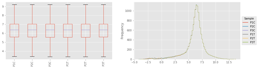
Visualise Normalized Counts
In [55]:
fig,axes=plt.subplots(figsize=(16,4),ncols=2)
ax = axes[0]
out_table.plot(kind='box',ax=ax,rot=90,showfliers=False)

ax = axes[1]
out_table.replace(-np.inf,-1.5).plot(kind='hist',
                                            histtype='step',
                                            bins=100,ax=ax)
UT.hist_legend(ax,'Sample')
#ax.set_xticklabels(out_df.columns, rotation=90, )
plt.show()
print(out_table.shape)
Differential Expression Analysis
In [72]:
%%R
library(edgeR)
# Make groups
design_with_all <- model.matrix( ~0+group )
y <- DGEList(counts=indata, group = group)
y <- calcNormFactors(y)

y <- estimateDisp(y, design_with_all)
# Estimate dispersion
# Fit counts to model
fit_all <- glmQLFit( y, design_with_all )
In [73]:
%%R
contrastCT <- glmQLFTest( fit_all, contrast=makeContrasts( groupT-groupC, levels=design_with_all ) )
tableCT <- topTags(contrastCT, n=Inf, sort.by = "none", adjust.method="BH")$table
head(tableCT)
In [110]:
%%R
t=topTags(contrastCT,n=20)
t$table
In [111]:
desc_dict['Tb08.27P2.90']
Out[111]:
In [74]:
%R -o tableCT

def mod_table(intable):
    intable['mlog10FDR']=-np.log10(intable['FDR'])
    intable['mlog10pvalue']=-np.log10(intable['PValue'])
    intable['desc']=[desc_dict.get(n,n) for n in intable.index.values]
    return intable

tableCT = mod_table(tableCT)
In [114]:
tableCT.sort_values('logFC').tail(10)
Out[114]:
In [ ]:
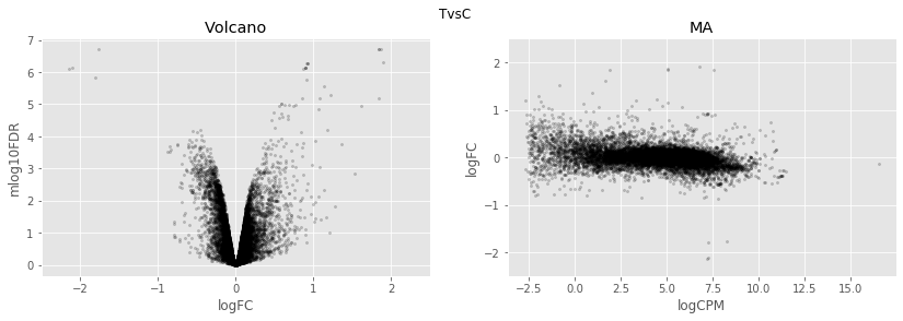
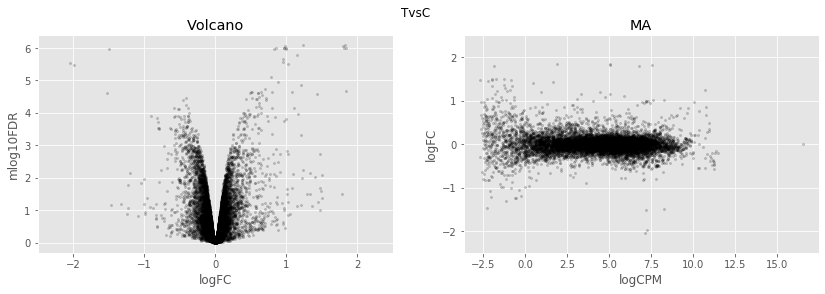
In [75]:
for table,name in zip([tableCT],
                 ['TvsC',]):

    fig,axes=plt.subplots(figsize=(14,4), ncols=2, nrows=1)
    ax=axes[0]
    table.plot(x='logFC',y='mlog10FDR',
           kind='scatter',s=5,alpha=0.2,ax=ax,c='black')
    ax.set_xlim(-2.5,2.5)
    ax.set_title('Volcano')
    ax=axes[1]
    table.plot(x='logCPM',y='logFC',
           kind='scatter',s=5,alpha=0.2,ax=ax,c='black')
    ax.set_ylim(-2.5,2.5)
    ax.set_title('MA')
    plt.suptitle(name)
    plt.show()
In [128]:
table.loc['Tb927.11.12100']
Out[128]:
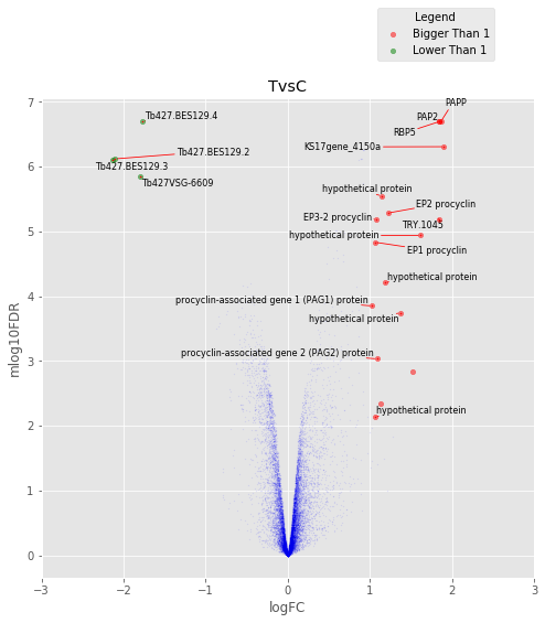
In [172]:
def annotated_volcano(table,name,selection=False):

    fig,axes=plt.subplots(figsize=(8,8), ncols=1, nrows=1)
    ax=axes
    if not selection:
        selection = table[((table['logFC']>1)|(table['logFC']<-1))
                          &(table['mlog10FDR']>2)&(table['logCPM']>0.8)]
    else:
        selection = table.loc[selection]
    annot_index = selection.index.values
    annot_names = selection['desc'].replace({'phosphatidic acid phosphatase protein  putative':
                                             'PAPP',
                                            'RNA-binding protein  putative':'RBP5',
                                            'PAP2 superfamily  putative':'PAP2',
                                            'THT1 - hexose transporter  putative':'THT1'})


    UT.make_vulcano(
        table,
        ax,
        x='logFC',
        y='mlog10FDR',
        fc_col = 'logFC',
        pval_col = 'FDR',
        pval_limit=0.01,
        fc_limit=1,
        annot_index=annot_index ,
        annot_names=annot_names,
        expand_text=(1.5, 1.5),
    expand_points=(2, 2),)
    ax.legend(loc='upper center', bbox_to_anchor=(0.8, 1.2), title='Legend')
    ax.set_xlim(-3,3)
    plt.title(name)
In [173]:
for table,name in zip([tableCT],
                 ['TvsC',]):
    annotated_volcano(table,name)
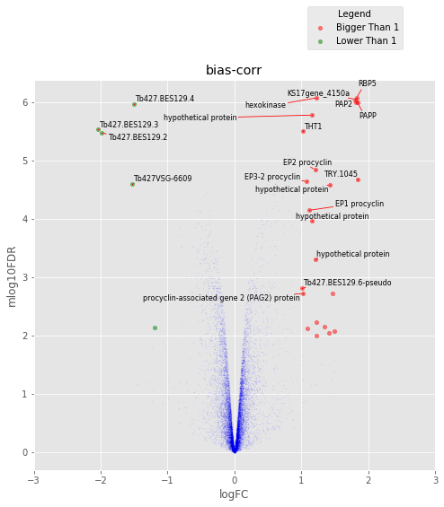
In [79]:
%%R
#https://rstudio-pubs-static.s3.amazonaws.com/79395_b07ae39ce8124a5c873bd46d6075c137.html
library(edgeR)
# Make groups
design_with_all <- model.matrix( ~0+group )

y <- DGEList(counts=indata,
                  lib.size = sizeFactors,
                  group = group,
                  )

y$offset <- cqn.subset$glm.offset
# Estimate dispersion
y <- estimateGLMCommonDisp( y, design_with_all )
y <- estimateGLMTrendedDisp( y, design_with_all )
y <- estimateGLMTagwiseDisp( y, design_with_all )
# Fit counts to model
fit_all <- glmQLFit( y, design_with_all )


#contrastDC <- glmLRT( fit_all, contrast=makeContrasts( groupD-groupC, levels=design_with_all ) )
#tableDC <- topTags(contrastDC, n=Inf, sort.by = "none", adjust.method="BH")$table
#head(tableDC)


contrastCT2 <- glmQLFTest( fit_all, contrast=makeContrasts( groupT-groupC, levels=design_with_all ) )
tableCT2 <- topTags(contrastCT2, n=Inf, sort.by = "none", adjust.method="BH")$table
head(tableCT2)
In [80]:
%R -o tableCT2
tableCT2 = mod_table(tableCT2)
In [174]:
annotated_volcano(tableCT2,'bias-corr')
In [150]:
for table,name in zip([tableCT2],
                 ['TvsC',]):

    fig,axes=plt.subplots(figsize=(14,4), ncols=2, nrows=1)
    ax=axes[0]
    table.plot(x='logFC',y='mlog10FDR',
           kind='scatter',s=5,alpha=0.2,ax=ax,c='black')
    ax.set_xlim(-2.5,2.5)
    ax.set_title('Volcano')
    ax=axes[1]
    table.plot(x='logCPM',y='logFC',
           kind='scatter',s=5,alpha=0.2,ax=ax,c='black')
    ax.set_ylim(-2.5,2.5)
    ax.set_title('MA')
    plt.suptitle(name)
    plt.show()
In [168]:
tableCT2[tableCT2['mlog10FDR']>4].sort_values('logFC').tail(20)
Out[168]:
In [146]:
tableCT2[tableCT2['mlog10FDR']>4].sort_values('logFC').head(5)
Out[146]:
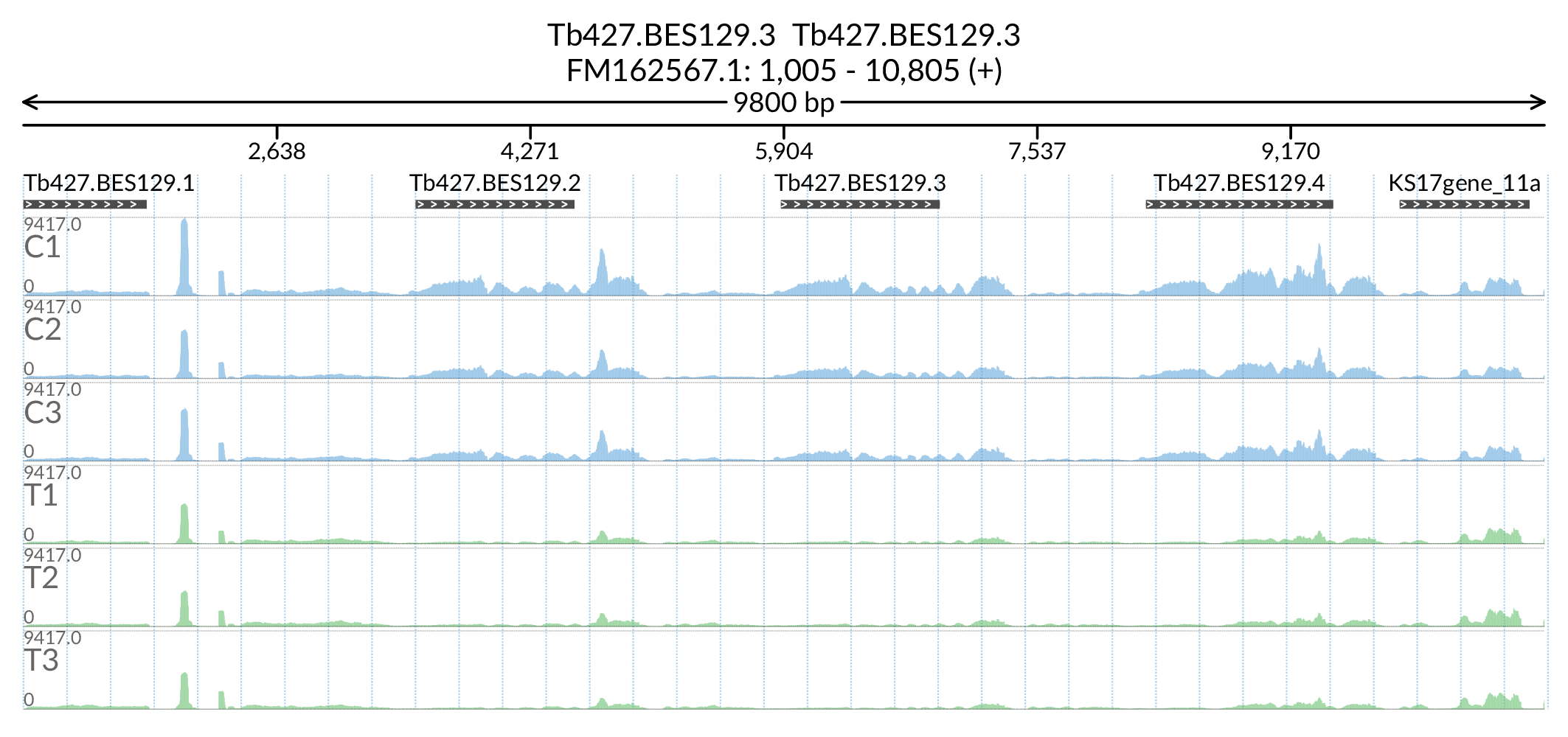
In [177]:
Image('Figures/Tb427.BES129.3_paperFig.png')
Out[177]:
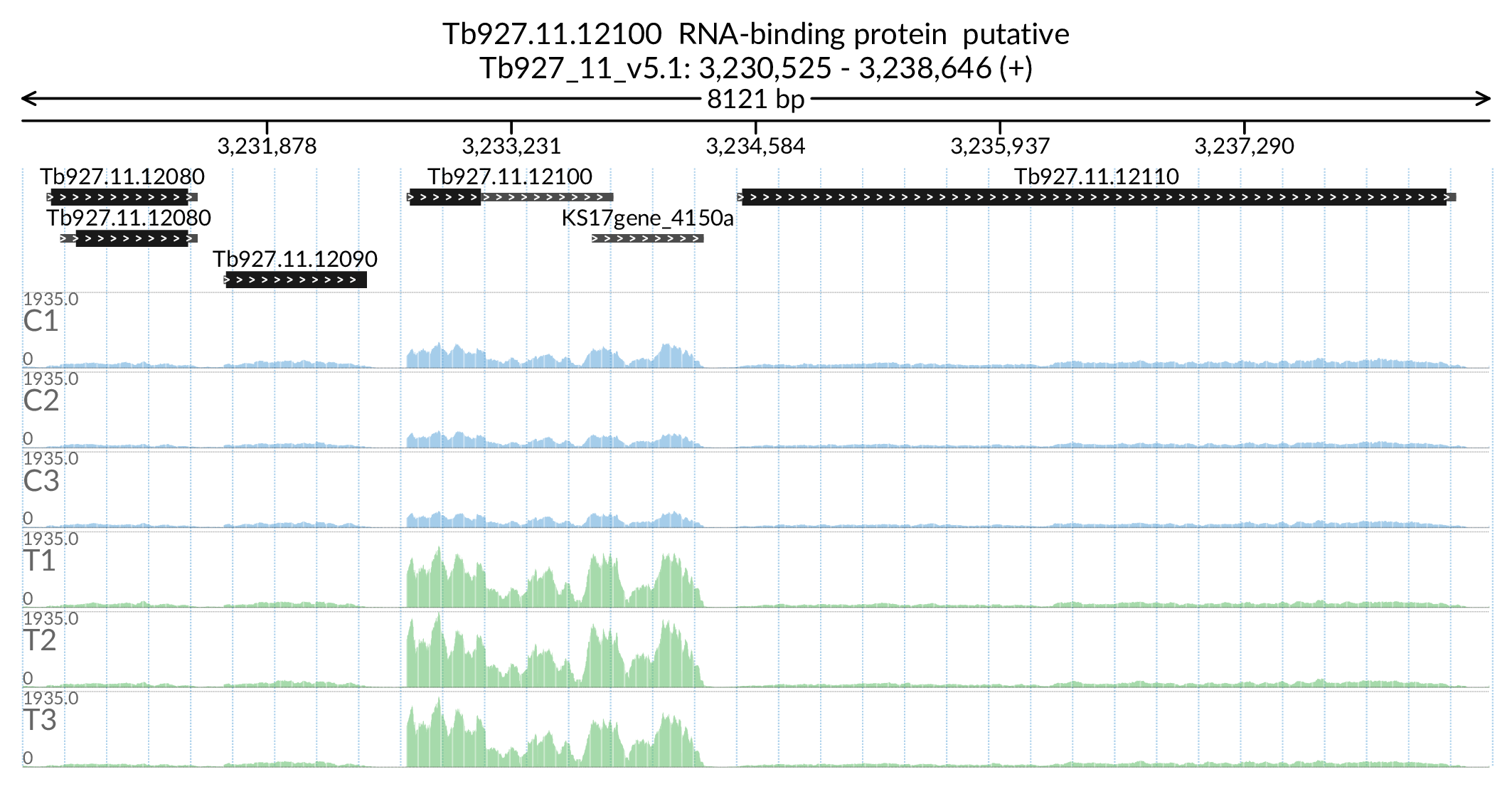
In [178]:
Image('Figures/Tb927.11.12100_paperFig.png')
Out[178]:
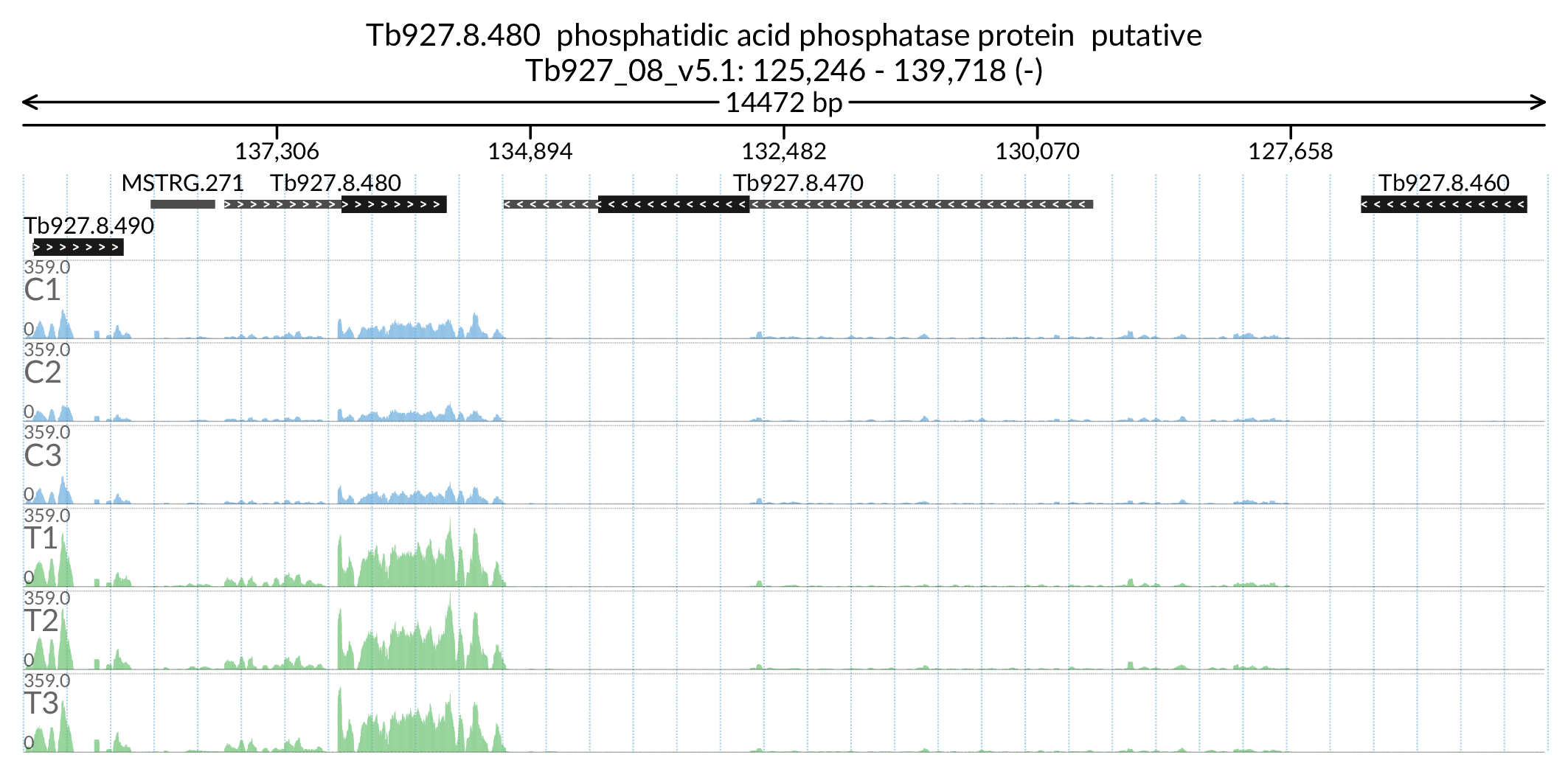
In [179]:
Image('Figures/Tb927.8.480_paperFig.png')
Out[179]:
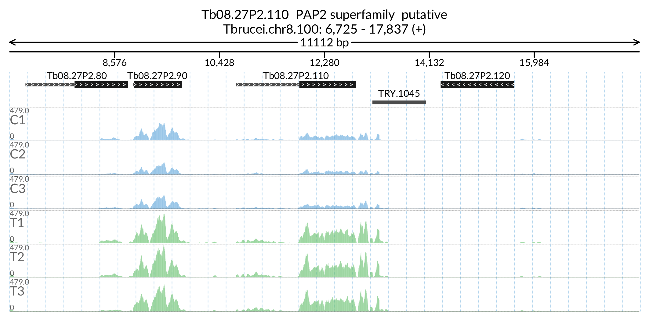
In [180]:
Image('Figures/Tb08.27P2.110_paperFig.png')
Out[180]:
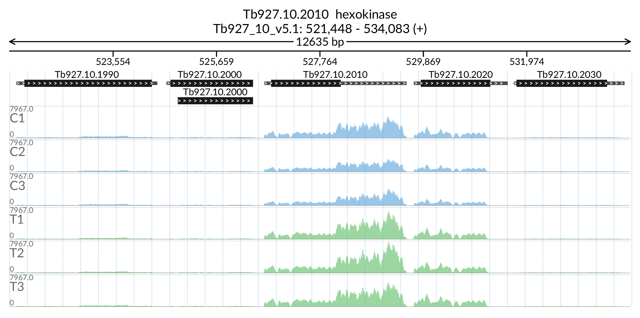
In [181]:
Image('Figures/Tb927.10.2010_paperFig.png')
Out[181]:
In [183]:
!jupyter nbconvert --to html_toc FiguresPaper.ipynb
In [ ]: